Data-Driven Machine-Learning Quantifies Differences in the Voiding Initiation Network in Neurogenic Voiding Dysfunction in Women With Multiple Sclerosis

Article information

Int Neurourol J. 2019;23(3):195-204

Publication date (electronic) : 2019 September 30

doi : https://doi.org/10.5213/inj.1938058.029

Christof Karmonik^,1,2, Timothy Boone¹, Rose Khavari¹

¹Department of Urology, Houston Methodist Hospital, Houston, TX, USA

²Translational Imaging Center, Houston Methodist Research Institute, Houston, TX, USA

Corresponding author: Christof Karmonik http://orcid.org/0000-0002-6695-9535 Translational Imaging Center, Houston Methodist Research Institute, 6565 Fannin, Houston, TX, USA E-mail: ckarmonik@houstonmethodist.org / Tel: +1-713-252-2661 / Fax: +1-713-441-7295

Received 2019 February 27; Accepted 2019 May 27.

Abstract

• HIGHLIGHTS

INTRODUCTION

As many as 90% of multiple sclerosis (MS) patients experience some sort of voiding dysfunction (VD) or incontinence [1]. The loss of neural conduction along axonal pathways that occurs in MS is caused by autoimmune-driven demyelination often accompanied by edema worsening the neurologic impairment. Depending on the affected regions in the central nervous system, symptoms vary greatly [2], generally characterized by neurogenic lower urinary tract dysfunction (NLUTD) [3] and may include difficulty of initiation or maintenance of voiding (VD).

Traditional clinical assessments such as urodynamic testing and urinary symptoms may not correlate with findings derived from standard clinical imaging [4]. Advanced neuroimaging methods, such as functional magnetic resonance imaging (fMRI) allow probing the involvement of regions in the brain and brainstem during micturition and have been recently successfully applied to female MS patients [5].

The demyelination of white matter tracts in MS affects functional connectivity (FC) in the brain [6]. A method to probe FC during micturition was recently presented [7]. In this approach, while undergoing a fMRI examination, subjects performed a voiding task during which blood oxygen level dependent (BOLD) signal time curves were recorded. Standard fMRI BOLD analysis provides a means to identify the brain network active during initiation of voiding. Strength of FC in this network is then derived from the degree of synchronicity of the BOLD signal time curves of corresponding voxels. The variation of FC in MS patients with VD may provide a more detailed picture of neural deficiency as it may directly relate to the underlying loss of anatomical connectivity while the activation/deactivation of a particular brain region alone (as assessed by traditional fMRI BOLD analysis) may constitute a consequence of this impaired connectivity.

Distribution of white matter lesions in MS visible in standard clinical images vary individually. Large-scale diffusional changes in normal appearing white and gray matter have been reported thereby attributing a neurodegenerative component to MS [8].

While these findings may not allow generalization of FC disruptions, we hypothesize that differences in the Voiding Initiation Network in VD versus spontaneous voiders will be discernible.

Machine-learning algorithms furnish the technical means to assess the predictive power of FC strength of selected brain regions in the Voiding Initiation Network in order to distinguish these 2 patient groups. From the FC analysis, a complex interaction between different brain regions is obtained, which is represented by the correlation coefficient of the fMRI BOLD time courses. With machine-learning, this complexity can be handled efficiently, where all the connectivity information is used directly, in the training and classification approach. In addition, once trained, the machine-learning algorithms used here will allow providing a relative importance for each brain region.

Identifying these brain regions may lead to improvement of therapy, in particular of new approaches that aim to use brain stimulation techniques aimed at cortical modulation [9].

MATERIALS AND METHODS

Voiding Initiation Brain Network in MS

The Voiding Initiation Network in MS was identified by the most highly activated voxels (t=3.5) in the averaged BOLD activation map and detailed in Supplementary material 1. This threshold was chosen as a compromise to include voxels in all pertinent brain regions, which exhibited activation in the averaged BOLD fMRI map (P<0.05), and at the same time to limit the number of predictor variables to render the data suitable for the machine-learning analysis. The resultant voxels (n=227) defined the brain network of voiding initiation (Fig. 1).

Fig. 1.

Upper panel: Voxels of the Voiding Initiation Network colored by functional magnetic resonance imaging blood oxygen level dependent activation overlaid onto brain anatomy in Talairach space. Lower panel: Individual and averaged functional connectivity (FC) patterns in the 27 multiple sclerosis patients participating in this study visualized by a color representation of the corresponding adjacency matrix (V, voider; VD, voiding dysfunction). In this presentation, vertices (i.e., voxels) of the Voiding Initiation Network are displayed vertically and horizontally. The intensity of the colored circle represents the strength of connection between each region (red: positive correlation, blue: negative correlation). As connections are undirected, the patterns are symmetric around the diagonal. While individual variation can be appreciated, VD globally exhibit weaker connections and larger variations. Consequently, while similar, the averaged FC pattern for VD is generally weaker and less coherent (lower right).

For each subject, a FC graph network was created using the voxels of the Voiding Initiation Network as vertices. Edge weights were defined as the correlation coefficient of the BOLD signal time courses of the corresponding voxels centered around its mean and divided by their standard deviation (R-project, scale function).

Graph networks were visualized by their adjacency matrix (R-project, corrplot package) and by their connectivity pattern in Talairach anatomical space (Paraview, Kitware Inc., Clifton Park, NY, USA).

RESULTS

Voiding Initiation Network in MS

Spatial extent

The Voiding Initiation Network in MS was found to be widely distributed in the brain including areas such as the dorsal vagal motor nuclei, pontine storage and micturition center, periaqueductal gray (PAG), ventral tegmental area, substantia nigra, red nuclei, thalamus, cingulate and insula was well as cortical regions in the frontal, parietal, and mesial temporal lobes (Fig. 1, Supplementary material 1). Visualization in the anatomical Talairach space demonstrates a global connectivity pattern: for frontal brain regions the connection strength was mainly positive while cerebellar regions and selected limbic regions were more negative (Fig. 2).

Fig. 2.

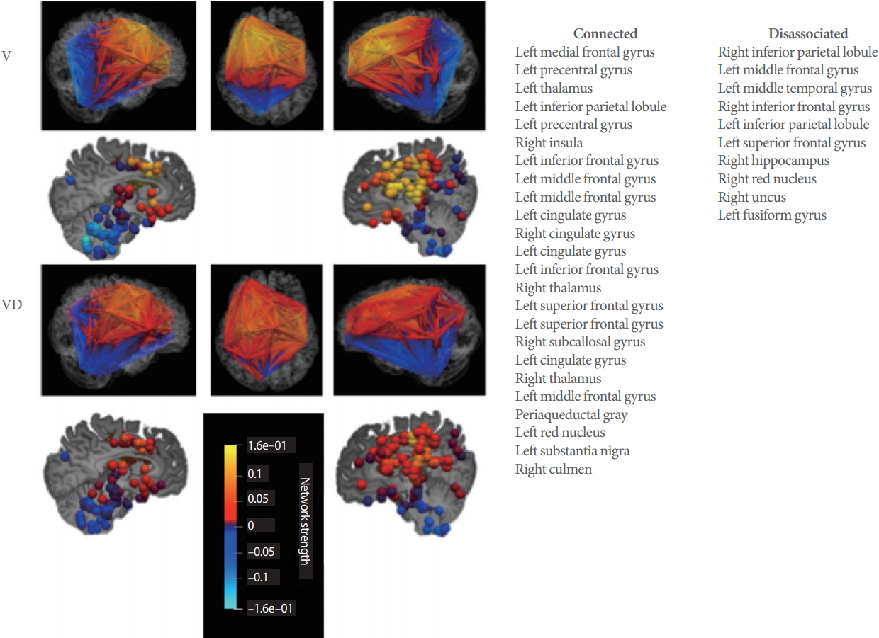
Averaged functional connectivity patterns for voiders (Vs) and voiding dysfunction (VD) from Fig. 1 displayed in anatomical space. Color is based on graph network strength of the individual vertices (voxels). Lower maximum strength in the VD network, particular in the frontal lobes and the cerebellum, can be appreciated. On right, brain regions are listed in 2 columns. The first column (connected) identifies voxels of the Voiding Initiation Network (by location) where total connection strength is positive for VD and negative for V. The second column (disassociation) lists those voxel of the Voiding Initiation Network (by location), where total connection strength is negative for VD and positive for V (see Supplementary material 1 for numerical values).

Differences between voiders and voiding dysfunction

While some variation existed between the individual networks, in general voiders exhibited stronger connections (Fig. 1). Similar to the individual networks, also the averaged network for voiders demonstrated stronger connections (Fig. 1).

Network components in the PAG, thalamus, substantia nigra, insula, subcallosal gyrus, hippocampus and in the frontal lobes were stronger connected for VD than voiders, whereas components in the temporal lobe hippocampus and fusiform gyrus were weaker connected for VD than voiders (Fig. 2, Supplementary material 1).

Machine-Learning Analysis

AUC values

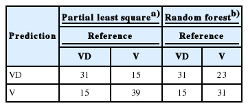
The 2 best-performing machine-learning algorithms were found to be partial least squares (AUC=0.89) and random forests (AUC=0.86) (Fig. 3). AUC for the Neural Network algorithm was 0.71 and worst performance the GLM (AUC=0.61) (Table 1).

Fig. 3.

Upper panel: Area under the curve (AUC) for all 4 machine-learning algorithms employed. AUC are provided. Lower panel: Receiver-operating characteristic curve (ROC) all 4 investigated machine-learning algorithms. Random forests (RF) and partial least squares (PLS) clearly outperform the other 2 algorithms. NNET, Neural Networks; GLM, generalized linear model.

Table 1.

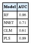
Area under the curve (AUC) values for the different models

Performance on test data sets

Evaluating the 2 best algorithms on the test data set yielded good values for accuracy (0.69 for partial least squares and 0.62 for random forests) (Table 2).

Table 2.

Confusion matrices for the 2 models (%)

Relative Importance of Brain Regions

For the best-performing machine-learning model (partial least squares), brain regions with highest importance were located in the frontal lobes and the cingulate (Table 3, Fig. 4). Other regions of high importance included the precentral and parahippocampal gyrus as well as regions in the cerebellum (Fig. 4). However, no real ‘cutoff ’ in the relative importance was observed, 25 regions showed importance higher than 70% and 186/227 voxels in the Voiding Initiation Network had a relative importance higher than 60% (Fig. 4, Table 3).

Table 3.

Relative importance (PLS) of first 30 most important voxels of the Voiding Initiation Network that differentiate between voiders and voiding dysfunction (Fig. 4)

Fig. 4.

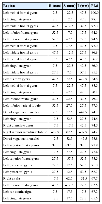
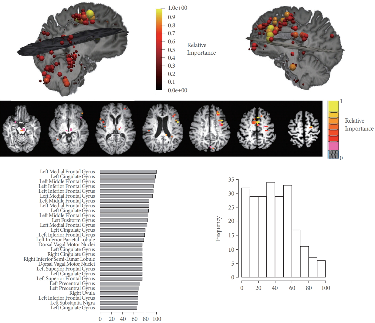
Upper panel: Relative importance differentiating functional connectivity (FC) in voiders and voiding dysfunction for vertices belonging to the Voiding Initiation Network displayed in anatomical space. Individual vertices corresponding to voxels in the brain are display in pseudo-color and size according the importance. Highest importance is found in the frontal lobes and cerebellum, but is generally high for all voxels. Middle panel: Voxel from top panel displayed in axial orientation in Talairach space. Lower panel: On left, the 30 top vertices (by location) of the Voiding Initiation Network with highest relative importance (in percent) in each hemisphere (coordinates are provided in Table 3). On right, histogram over all 227 voxels demonstrating the high relative importance for a large number of these voxels supporting the conclusion that FC is affected globally.

DISCUSSION

Our results demonstrate that patients with VD exhibit an altered functional connectome in their Voiding Initiation Network where largest variations relative to voiders are found in the frontal lobes and the cingulate.

Earlier neuroimaging studies have identified brain regions directly involved in initiating or continuing voiding in healthy individuals. These regions include: precentral gyrus, supplementary motor area, dorsolateral prefrontal lobe, inferior frontal gyrus, cingulate gyrus, insula, hypothalamus, PAG, and pons (PMC) [9-12], specifically the cingulate region is highly activated at full capacity and with strong desire to void (immediately prior to voiding) in healthy and MS patients [10-13]. Frontal and prefrontal regions of the brain combine all the input from cingulate, insula and hypothalamus and further the decision to void is made when it is the right time, the right place and with appropriate bladder volume [14,15].

Due to the diffuse, multifocal disease involvement of the brain in MS, anatomical connectivity and therefore FC is thought to be impaired on a global level [8]. Individual differences in the urinary symptom severity and impact on quality of life exist. This clinical observation is in concordance with our findings of global impairment of the Voiding Initiation Networks for VD patients compared to voiders. It is also in agreement with a reduction in similarity of the global FC patterns with disease progression reported recently [7].

Our approach complements standard clinical testing and established traditional fMRI BOLD techniques, which focuses solely on activation of brain regions. By being able to characterize the global FC connectome, our method allows monitoring FC changes with disease progression as well as therapeutic interventions. Of the latter, noninvasive brain stimulation has gained interest recently. It constitutes a promising new intervention in MS that has already yielded promising results for motor and cognitive function in combination with appropriate training exercises [9]. Identifying potential brain regions as target for stimulation (e.g., frontal regions) and monitoring global FC changes during and after stimulation may be essential for optimizing stimulation techniques.

Machine-learning algorithms have found recent applications in correlating clinical neuropsychological findings with brain connectivity measures. Examples include brain-computer interface stroke rehabilitation [11,12], discrimination of schizophrenia [13] and mild traumatic brain injury [14,15]. In contrast to these approaches, in our method, no assumptions are made about significance of connections by applying a threshold. Instead, the entire functional connectome of the Voiding Initiation Network is used as input into the machine-learning algorithms thereby improving the data-driven nature of the paradigm.

The number of subjects (n=27) for a machine-learning approach is somewhat limited, in particular, if compared with the number of predictor variables (i.e., number of brain voxels of the Voiding Initiation Network). The use of advanced algorithms, such as partial least squares or neural networks, where the original predictor variables are combined, thereby reducing the dimensionality of the predictor space, creates a more favorable ratio between this number of variables and the number of available data for training the algorithm. This in turn will help to arrive at a better trained algorithm. Such an approach therefore successfully addresses the limited number of clinical datasets, as they often exist in a single center clinical study. Alternatively, the machine-learning algorithm may be trained by combining data from several clinical sites. Once trained, it can then be applied to any single center study.

Two algorithms, random forests and partial least squares performed best according to their AUC values (0.86 and 0.89, respectively). Therefore, we conclude that these 2 algorithms are best suited for the classification problem in this study.

Understanding supraspinal centers and their role in initiating or modulating voiding is currently still limited in patients with neurogenic VD. By combining new concepts of neuroimaging with powerful machine-learning algorithms, we increase the knowledge of these processes and aid in phenotyping patients for novel treatment approaches such as brain stimulation.

In conclusion, machine-learning is capable of quantifying FC differences in MS patients with NLUTD and VD. The functional connectome of the Voiding Initiation Network is less coherent in this patient group. Global differences were found with focal points in the frontal lobes and the cingulate.

SUPPLEMENTARY MATERIALS

Article information Continued